Flowchart for the Analysis of Multi-Wavelength Sedimentation Velocity Data
Step 1: Import Experimental data into UltraScan-III OpenAUC format
Note
Required for data from XLA or XLI, this step is performed automatically in the Optima AUC. Sedimentation velocity data should not be measured in absorbance mode, use intensity mode instead.
Import the experimental data: Utilities: Import Experimental Data
Confirm Investigator setting and local/database selection
Import Experimental Data from local disk
Edit Run Information, Select Lab/Rotor/Calibration
Enter a Label (verbose description for the run)
Select the corresponding project by clicking on the Project button. If there is no project, create a new project.
Confirm experiment type and optical detection system
Enter any comments, if applicable
Select instrument, rotor, rotor calibration and operator
- Click on Accept.
Edit the Description field if necessary
Navigate to the first channel and select the centerpiece type.
- Select the proper solution - Make sure that the solution contains at least one analyte and a buffer
If you have more than one Triple, you can click on Apply to All but verify centerpiece and solution for each Triple first. Also, check the Description field again to make sure the appropriate information is saved.
If data were collected in intensity mode, you will need to Define Reference Scans by selecting a short region from the air-to-air interface portion of the data.
For equilibrium data from 6-channel centerpieces you should separate each channel with the Define Subsets/Process Subsets functions.
Failed Triples or empty Triples can be excluded from the run by clicking on Drop Selected Triples.
When everything has been set you can Save the scans to database or disk.
Step 2: Edit experimental data
Edit the data in the Edit Data module.
Load data from the database or a local data directory containing the UltraScan-III openAUC data files.data.
Select the Cell / Channel / Wavelength Triple to be edited.
Specify the meniscus of the data by holding down the Control key and using the left mouse button. The meniscus value may be manually adjusted with the keyboard.
Specify the left and right edges of the data to be analyzed.
Note
Please note: Do not pick the left data edge too close to the meniscus. During meniscus fitting, the evaluated meniscus positions may reach inside of the data range and violate the boundary conditions of the finite element solution. This will cause the meniscus fit to fail.
Specify the location of the scan plateau. This is the radial position where most scans have a stable plateau, but the selected position should not reach into the back-diffusion region. The most appropriate point tends to be close to the right edge of the data range, but not so far to the right that it extends into the region where the concentration of the later scans curves upward at the bottom of the cell due to back-diffusion.
Make any other optional adjustments to the data that are necessary and save the edit profile. When saving, a pop-up message is presented asking for an edit ID. The default for this ID is the current date and time in the form of YYMMdd hhmm (Year / Month / Day / Hour / Minute), but this default can be supplemented with a suffix of your own choice.
Step 3: Inspect and plot the raw data
Inspect the raw MWL data using the Multi-Wavelength Raw Data Viewer in the Multi-wavelength modules.
Load the data from the local disk or the database.
Select the Cell / Channel / Wavelength Triple to be inspected.
Generate and save the 3-D plot and movie.
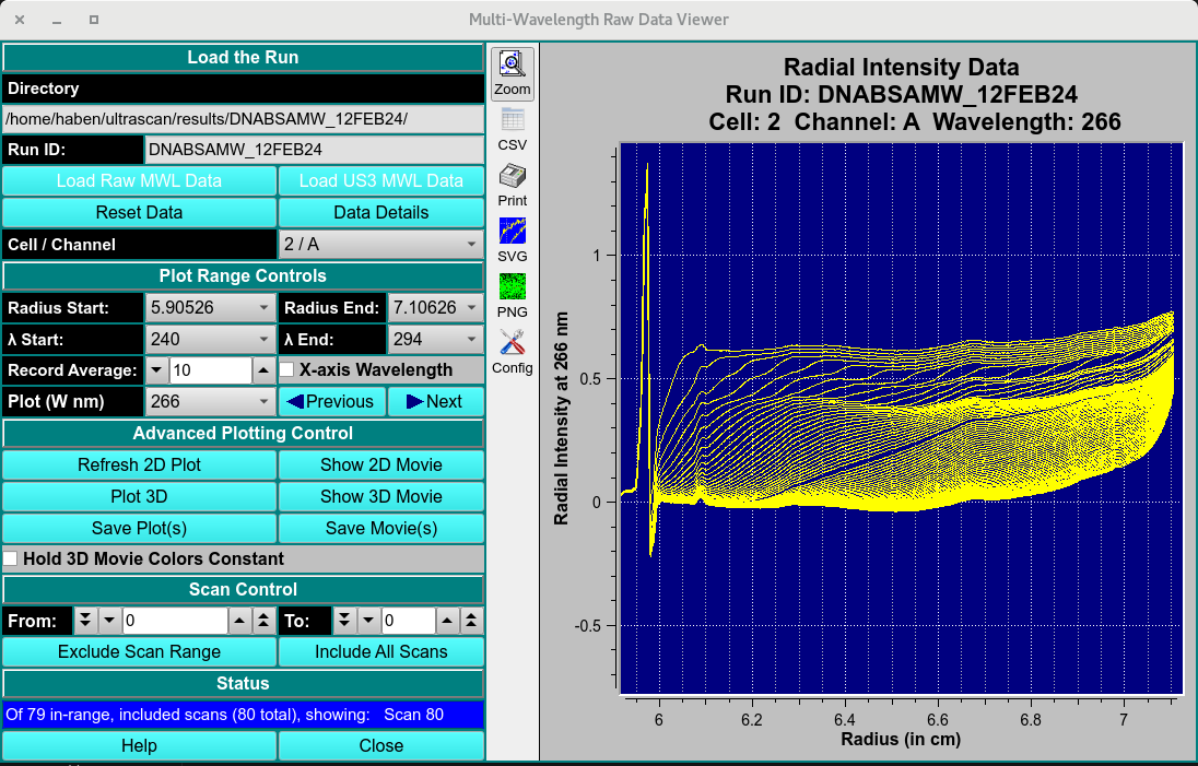
Raw MWL Data Inspection and Plotting
Step 4: Perform a 2DSA refinement following the 2DSA Flowchart
Follow Steps 3-6 in the 2DSA Flowchart to perform 2DSA analysis and fit the associated Time- and Radially- invariant noises, the meniscus and bottom boundary positions and rotor stretching and final iterative refinements.
Step 5: Simulated a time-grid synchronized model based on 2DSA-IT MWL models
Simulate a time synchronized ISSF_ model based on the MWL 2DSA-IT models using the MWL Pre-Fit Species Simulation.
Click PreFilter Models to define the MWL pre-filter for the simulation and
Click Select Models and load all related 2DSA-IT models from one MWL dataset channel.
Define Buffer and open the Buffer Management dialog to define the experimental parameters of the dataset
Define the simulation parameters
Click Define Rotor and open the Rotor Management dialog to select the Default 1003 (Simulation) rotor.
Start the simulation and save the open-auc file into $HOME/ultrascan/imports folder.
Step 6: Create basis spectra for each species
Generate the extinction coefficient basis spectrum of an analyte in the Spectrum Fitter dialog.
Using a UV-visible spectrophotometer, scan the serial dilutions of analyte - spectra.
load csv files, define the column separator character and click Apply.
Add the extinction coefficient of the analyte at 260 or 280 nm, and click Perform a global fit if known.
A second fitting dialog will appear to perform the fit. Typical users don’t have to change any setting. Click Fit.
Once the fit is complete, the result will automatically populate the main window. On the main window, click Save. Give the .dat file a unique name.
Step 7: Import and Edit the ISSF- data file
Repeat steps 1 and 2 for the newly generated ISSF- open auc file.
Step 8: Deconvolute MW data using species basis spectra
Deconvolute the analytes in MWL Species Fit Analysis.
Load the time-synchronized ISSF- simulation generated using Optima MWL Fit Simulations using Load Run Data Dialog .
Click Load Species Fits and load the species extinction coefficient basis spectra from local disk.
Perform the deconvolution by clicking Species Fit Data.
Deconvoluted sedimentation velocity data of each species will by generated with a SSF-ISSF- pre-fix.
Step 9: Import and Edit the SSF-ISSF- data files
Repeat steps 1 and 2 for the newly generated SSF-ISSF- open auc files.
Step 10: Perform a 2DSA with refinement only
Perform 2DSA refinement of the SSF-ISSF- datasets.
Step 11: Perform van Holde-Weischet analysis - (recommended)
Open Velocity: Enhanced van Holde-Weischet.
Load the desired experiment, applying the noise files from Step 6 (the latest model).
Check Plateaus from 2DSA and Use Enhanced vHW.
Adjust Beck Diffusion Tolerance, Divisions, Data Smoothing, % of Boundary, and Boundary Position to desired values.
If appropriate, delete early scans to improve resolution and reduce noise. Only keep scans and boundary portions that contribute to well correlated line fits in the linear extrapolations.
Select groups, if appropriate, to generate weight averaged s-values for discrete species.
Display Distribution Plot and histogram.
Save Data and distributions.
Note
Refer to the van Holde-Weischet manual page for additional details.
Step 12: Overlay combined distributions - (recommended)
All van Holde-Weischet distributions and finite element models can be combined into a single plot for easy comparison.
Use Velocity: Combine Distribution Plots (vHW) for van Holde-Weischet plots.
Use Velocity: Combine Discrete Distributions for all finite element models (2DSA, GA, Monte Carlo).
Use Velocity: Combine Integral Distributions for all finite element models (2DSA, GA, Monte Carlo).
Use Velocity: Combine pseudo-3D Distributions for all finite element models (2DSA, GA, Monte Carlo).
Reference
2DSA
Brookes E, Cao W, Demeler B. A two-dimensional spectrum analysis for sedimentation velocity experiments of mixtures with heterogeneity in molecular weight and shape. Eur Biophys J. (2010) 39(3):405-14.
Kim H, Brookes E, Cao W, Demeler B. Two-dimensional grid optimization for sedimentation velocity analysis in the analytical ultracentrifuge. Eur Biophys J. 2018 Oct;47(7):837-844. doi: 10.1007/s00249-018-1309-z. PMID: 29777290
Experimental Design
Demeler, B. (2024). Methods for the design and analysis of analytical ultracentrifugation experiments. Current Protocols, 4, e974. doi: 10.1002/cpz1.974
PCSA
Gorbet G., T. Devlin, B. Hernandez Uribe, A. K. Demeler, Z. Lindsey, S. Ganji, S. Breton, L. Weise-Cross, E.M. Lafer, E.H. Brookes, B. Demeler. A parametrically constrained optimization method for fitting sedimentation velocity experiments. Biophys. J. (2014) vol 106, 1741-50.
Genetic Algorithm
Brookes E, Demeler B. Parsimonious Regularization using Genetic Algorithms Applied to the Analysis of Analytical Ultracentrifugation Experiments. GECCO ‘07: Proceedings of the 9th annual conference on Genetic and evolutionary computation, London, July 7-11, 2007, 361–368, https://doi.org/10.1145/1276958.1277035, ACM 978-1-59593-697-4/07/0007
Monte Carlo
Demeler B and E. Brookes. Monte Carlo analysis of sedimentation experiments. Colloid Polym Sci (2008) 286(2) 129-137
Adaptive Space-Time Finite Element Solution
Cao, W and Demeler B. Modeling Analytical Ultracentrifugation Experiments with an Adaptive Space-Time Finite Element Solution for Multi-Component Reacting Systems. Biophys. J. (2008) 95(1):54-65